Understanding Vector Embeddings and how to work with them in PEACH
Introduction to embeddings
Vector embeddings are numerical representations of data that capture the inherent characteristics and relationships between items in a high-dimensional space. They play a crucial role in various machine learning tasks, enabling systems to understand and process complex information more effectively.
What are Vector Embeddings?
At its core, a vector embedding is a set of numbers arranged in a particular order. Each number in the set represents a feature or aspect of the item being encoded. By arranging these numbers in a specific way, embeddings can encode rich information about the item's attributes, context, and relationships with other items.
How are Vector Embeddings Computed?
Vector embeddings are often computed using machine learning models, such as encoder Transformer architectures like BERT, GPT, or similar techniques. These models are trained on vast amounts of data to learn meaningful representations of input items and learn to "understand" the content.
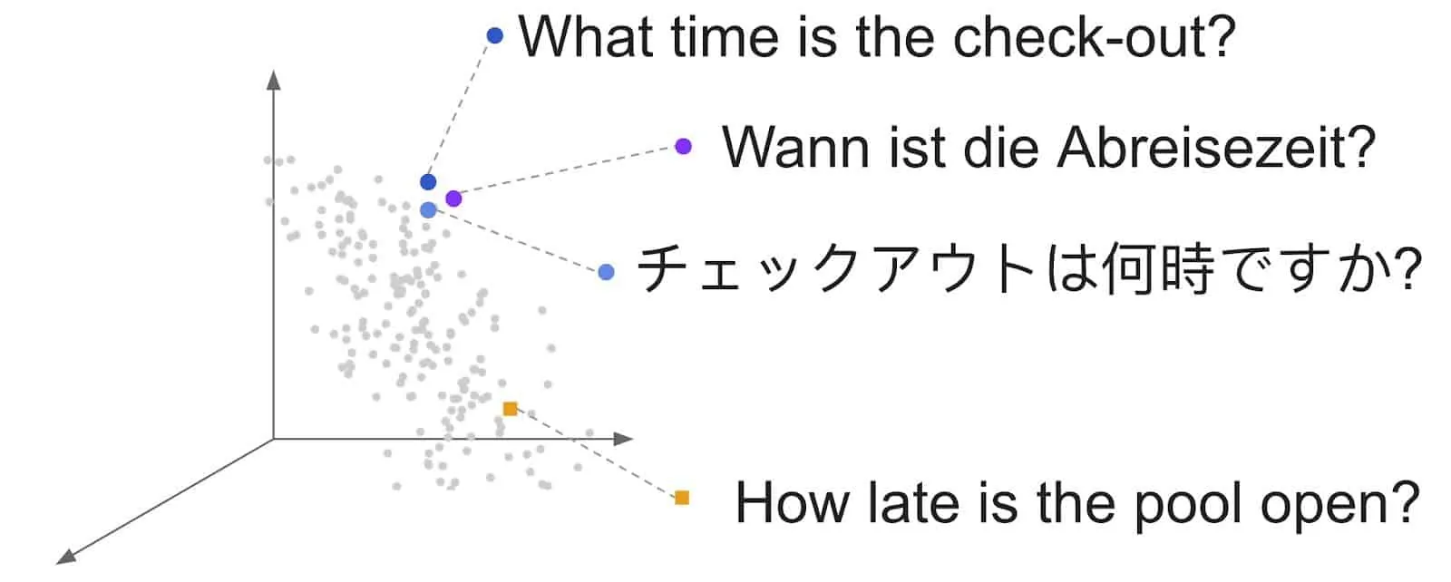
During training, the model learns to map input items, such as text, images, or audio, to dense numerical vectors in a high-dimensional space. This mapping process captures semantic similarities between items, allowing similar items to be closer together in the embedding space.
An important paper from Google Brain that introduces Transformers architecture is worth to get familiar with: Attention Is All You Need, as it became a foundation for a lot of recent progress in the field.
What Can Vector Embeddings Be Used For?
Vector embeddings have diverse applications across various domains, including:
- Semantic Similarity: Embeddings enable systems to measure the semantic similarity between items. For example, in natural language processing, embeddings can capture the similarity between words, sentences or even longer texts based on their semantic meaning.
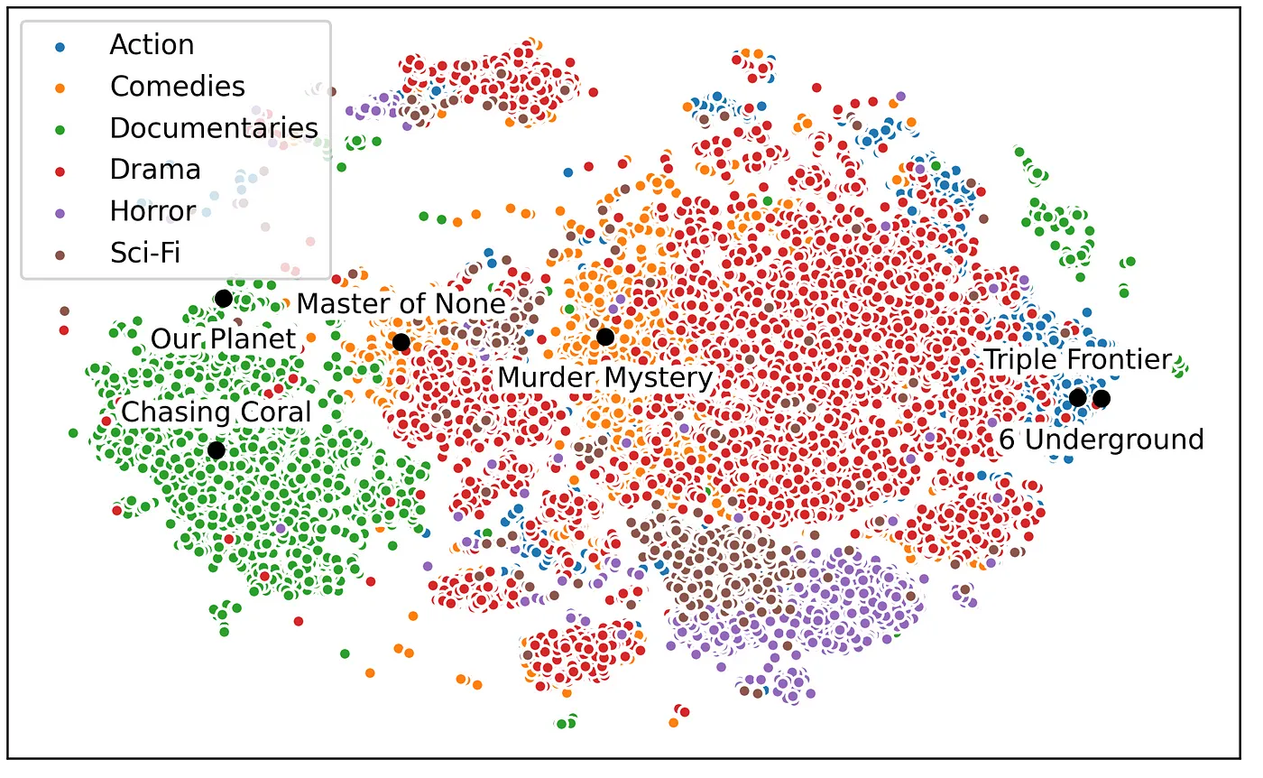
- Recommendation Systems: Embeddings power recommendation systems by representing items and users in a unified embedding space. Similar items or users are clustered together, enabling personalized recommendations based on similarity of content or user tastes.
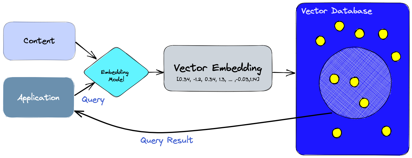
- Search and Retrieval: Embeddings facilitate efficient search and retrieval of similar items. By indexing embeddings in a database like Milvus, systems can quickly retrieve items that closely match a given query.
- Clustering and Classification: Embeddings can be used for clustering similar items together or classifying items into predefined categories. This is particularly useful in tasks like image recognition and document classification.

Examples of Vector Embeddings
-
Word Embeddings: In natural language processing, word embeddings represent words as dense vectors in a continuous space. Words with similar meanings are mapped to nearby points in the embedding space. Example: Word2Vec, GloVe.

-
Document Embeddings: Document embeddings capture the semantic content of entire documents, enabling systems to compare and retrieve similar documents. Example: Doc2Vec, BERT, Universal Sentence Encoder, Language-agnostic BERT Sentence Embeddings or some of LLM-based embeddings.


-
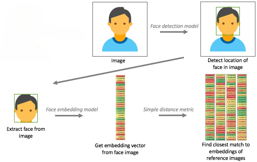
Image Embeddings: Image embeddings encode visual features of images, allowing systems to recognize similar images or detect visual patterns. Another common scenario is facial recognition. Example: Convolutional Neural Network embeddings.

-
Audio Embeddings: Audio embeddings represent audio signals as numerical vectors, enabling tasks such as speech recognition and audio classification. Example: VGGish embeddings for audio classification.
Why Vector Database?

- Efficient Storage: Vector databases are specifically designed to store and manage high-dimensional vector data efficiently. Traditional relational databases are not optimized for this type of data, leading to suboptimal performance and scalability issues when dealing with large-scale vector datasets.
- Fast Retrieval: Vector databases employ specialized indexing structures and algorithms tailored for similarity search tasks. These optimizations enable fast retrieval of nearest neighbors for a given query vector, even in high-dimensional spaces.
- Scalability: As the size of the dataset grows, performing brute-force similarity search becomes increasingly impractical due to its computational complexity. Vector databases are designed to scale efficiently with large volumes of vector data, allowing for real-time or near-real-time retrieval of similar items even on tens of millions of embeddings
- Approximate Nearest Neighbors (ANN): Vector databases often support approximate nearest neighbor search algorithms, which trade-off a small degree of accuracy for significant gains in search speed. These algorithms provide fast and scalable solutions for similarity search tasks, making them suitable for many real-world applications.
In PEACH we adopted open-source vector database Milvus, which is currently powering a lot of different usecases for PEACH members.
How to use Milvus in PEACH
First install the correct version of pymilvus, any 2.3.x version should suffice:
pip install pymilvus==2.3.5
Now let's set correct environment variables (they will already be setup for your organisation's tasks and endpoints environment, just need to do in PeachLab) and learn how to connect with the client:
import os

from pipe_algorithms_lib.similarity_2 import connect

os.environ['CODOPS'] = 'ltlrt'  # codops of your organisation
os.environ['CODOPS_LTLRT_MILVUS_PASSWORD'] = 'xxx'  # secret for your organisation. Already configured for tasks and endpoints. Contact PEACH Core team if you don't have it yet. Make sure to not push secret to git!

# needs to be executed only once. So for endpoints - better to move it out from inside your endpoint entry point function
connect()
Then, let's create schema for our embeddings collection. Milvus allows us to add fields in addition to just vector fields, so we can later query data not just based on vector similarity, but also to filter items based on other metadata fields (common fields could be category, publication_date, language, etc).
We should also create required indexes, to get the most optimal querying performance. You need to ensure that this code is executed once, as we don't want to create new collection for each task execution:
from pymilvus import DataType, FieldSchema

from pipe_algorithms_lib.similarity_2 import create_collection


create_collection(
    collection_name=COLLECTION_NAME,
    dimension=768,
    extra_fields=[
        FieldSchema(name='publication_date', dtype=DataType.INT64),
        FieldSchema(name='language', dtype=DataType.VARCHAR, max_length=16),
        FieldSchema(name='category', dtype=DataType.VARCHAR, max_length=255),
    ],
    indexes={
        'vec': {
            'metric_type': 'IP',
            'index_type': 'HNSW',
            'M': 32,
            'efConstruction': 128,
        },
        'publication_date': None,
        'language': None,
        'category': None,
    }
)
Here we create scalar indexes for all non-vector fields (if we plan to query based on them, but we can always add them later separately) and a vector field index. We use an HNSW index type with some reasonable hyperparameters, but don't hesitate to tune parameters as appropriate. You can read more on different vector index types and their hyperparameters here.
Once our collection has been created in your namespace, you can now insert documents into it:
from random import random
from datetime import datetime

from pipe_algorithms_lib.similarity_2 import index

# normally comes as output from an embedding model, but let's use a random vector for now
vector = [random() for _ in range(768)]

document = {
    'id': 'my_document_42',
    'vec': vector,
    'publication_date': int(datetime(2024, 3, 1, 12, 0, 0).timestamp()),
    'language': 'en',
    'category': 'sports',
}

# here we simply insert a single document. If you have many documents to index - better to send them in larger batches
documents_to_index = [document]

index(
    collection_name=COLLECTION_NAME,
    data=documents_to_index,
    normalize=True,  # whether to normalize input vectors. Usually required if using Cosine Similarity
    upsert=True,  # if upserting - then we override data by `id` to avoid duplicates
    flush=True,  # enabling flushing would make insert slower but we can be sure that data is now queryable
    timeout=5,
)
If we want to retrieve some documents (to get some metadata for a current item quickly or to get vectors for clustering, for example):
from pipe_algorithms_lib.similarity_2 import get_documents

document = get_documents(COLLECTION_NAME, ['my_document_42'], output_fields=['id', 'language', 'vec'])

# document -> {
#   'id': 'my_document_42',
#   'language': 'en',
#   'vec': [-0.041, 0.214, 0.012, -0.112, ...]
# }
And the most important step is actually querying the data, for find the most similar items to a given vector (useful to use some meaningful embeddings encoder and to have more items in the collection):
from pipe_algorithms_lib.similarity_2 import retrieve_similar

filter_expr = 'language == "fr" and publication_date >= 1704067200'

recs = retrieve_similar(
    COLLECTION_NAME,
    ids=['my_document_42'],  # if you pass multiple IDs - it finds mean vector from all the input vectors and finds similar to it
    size=10,
    filter_expr=filter_expr,
)

# alternatively, you can pass query vector instead of `ids`, if you want to find similar vectors without inserting current document into the database
recs = retrieve_similar(
    COLLECTION_NAME,
    query_vectors=[vector],
    size=10,
    filter_expr=filter_expr,
)

# recs -> [
#   {'id': 'my_document_42', 'distance': 0.99999},
#   {'id': 'my_document_73', 'distance': 0.86124},
#   {'id': 'my_document_14', 'distance': 0.74124},
#   ...
# ]
Conclusions
- Vector embeddings are powerful tools for representing and understanding complex data in machine learning applications. By capturing semantic similarities between items in a high-dimensional space, embeddings enable tasks such as recommendation, search, clustering, and classification to be performed efficiently and effectively.
- Vector databases like Milvus provide efficient storage, fast retrieval, scalability, and support for approximate nearest neighbor search algorithms, making them indispensable tools for content-based similarity search and recommendation systems in various domains. They offer significant advantages over brute-force search methods, enabling organizations to build high-performance and scalable solutions for similarity-based tasks.
- We learned how to interact with existing Milvus setup within PEACH environment, how to create collection with defined schema and indexes, add vectors with metadata and query for similar vectors, representing semantically similar content